Laser scanning imaging basics
Unlike wide-field microscopes, which collect full-field images simultaneously through flood illumination and cameras, laser scanning microscopes usually can only use single-focus illumination at a given time and restart after completing a line-by-line raster scan (Raster Scan). Composition image. Raster scanning is generally achieved through two mirrors (biaxial galvanometers). In the lower right image, the fast mirror scans along the x-axis and the slow mirror advances line by line.

Laser scanning imaging is not inherently superior to wide-field imaging, but higher-level imaging technologies can be used through laser scanning, and confocal and multiphoton are the two types that will be introduced in this article. Confocal imaging produces high-resolution images by suppressing light outside the focus, allowing three-dimensional images to be reconstructed through optical sectioning, while two-photon imaging has a very large depth.
Laser Scanning Engine: Mutual Constraints of Specifications
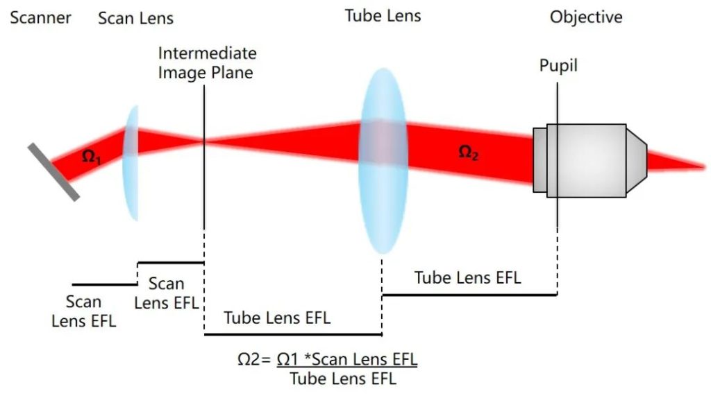
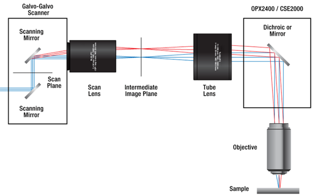
The four main optical components of the scan engine are the scanning mirror (galvanometer), scanning lens, tube lens and objective lens. The scanning mirror is located on the back focal plane of the scanning lens, and the distance between the scanning lens and the tube lens is equal to the sum of the front focal length of the scanning lens and the back focal length of the tube lens. Although the tube lens outputs a collimated beam and the objective lens is in the infinity correction space, so the distance between the two is not so strict, it is best to make the front focal plane of the tube lens coincide with the rear focal plane of the objective lens.
The following figure shows the relative position of each component and the relationship between the scanning angle. The angle of the scanning mirror Ω1 will be reduced to Ω2 according to the magnification of the scan engine, which is the angle at which the beam enters the objective lens.
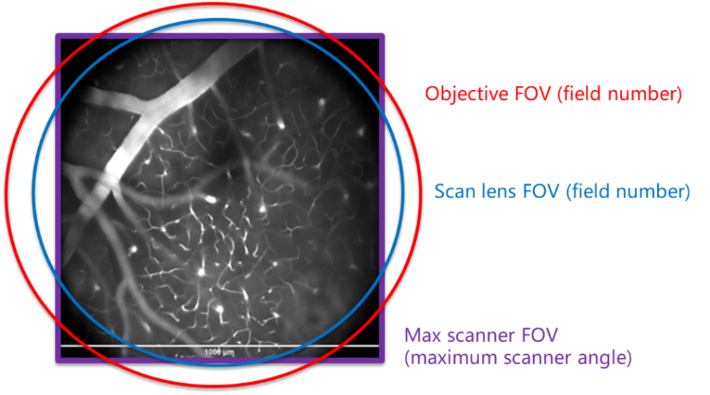
The field of view of a scan engine is often limited by the scanning optics rather than the objective lens. The scanning mirror not only has the largest off-axis angle, but also because raster scanning usually produces a square scanning area, which is the purple box in the figure below, while the fields of view of the scanning lens and objective lens are circular, respectively represented in the figure below Blue and red circles.
If the magnification of the scanning lens and tube lens is 1, although this will not reduce the angle at which the beam enters the objective lens, it will limit the maximum beam size entering the objective lens, preventing it from filling the rear aperture of the objective lens and reducing the resolution. This is because the objective rear aperture is filled with uniform flat-top light to achieve diffraction-limited resolution. Furthermore, axial resolution is more affected by this than lateral resolution.
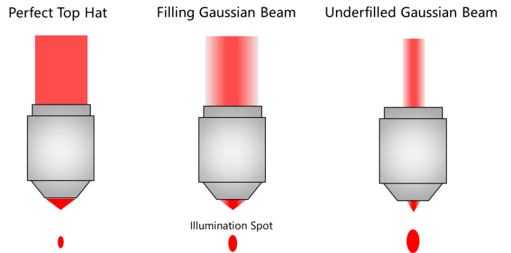
In addition, real samples can also introduce scattering and wavefront distortion, causing defocus. This problem may be related to numerical aperture. For biological tissues with large variations in refractive index, light incident from high numerical apertures may cause destructive interference at the focus, disrupting the wavefront and enlarging the focal spot. Unfilled objectives may not have these high numerical aperture rays and therefore provide a better wavefront and smaller focal spot.
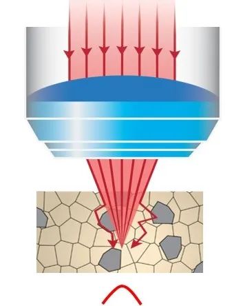
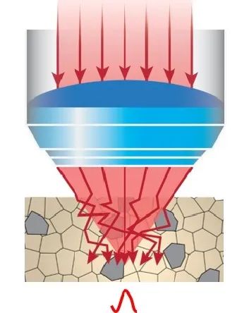
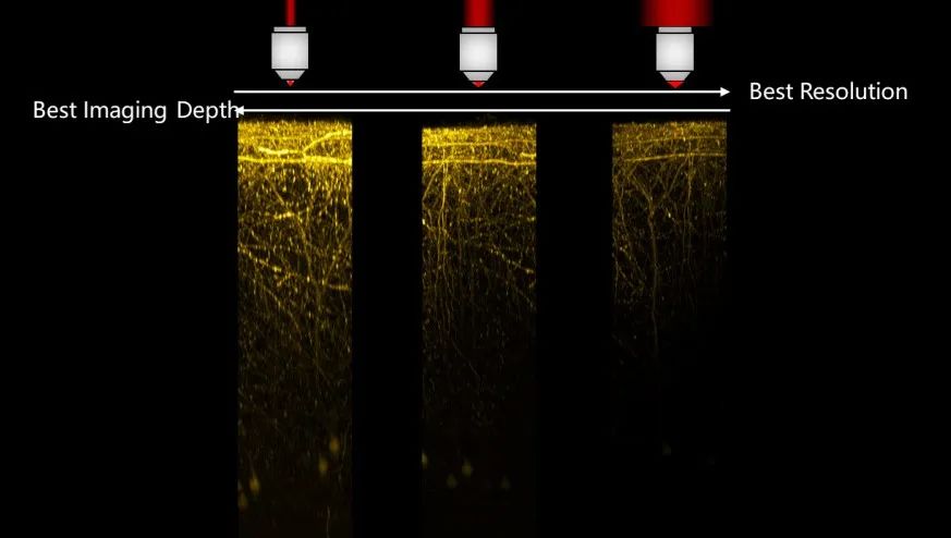
Therefore, resolution and imaging depth are also two factors that restrict each other. The relationship between the two is vividly displayed in the figure below. Overfilling the objective lens with the beam can produce high-resolution images near the tissue surface, but cannot image very deep into the tissue due to scattering and other wavefront errors. When the beam does not fill the objective lens, it has low resolution but produces a deeper image.
Scan Engine: Properties of Main Components
Before introducing each scanning component, let’s take a look at the scanning engine design specifications of the multiphoton microscope:
| Clear Aperture Diameter | × | Beam Magnification | = | Max Beam Size |
| 5 mm (Galvo-Resonant) | × | 4 | = | 20mm |
| 4 mm (Galvo-Galvo) | × | 4 | = | 16mm |
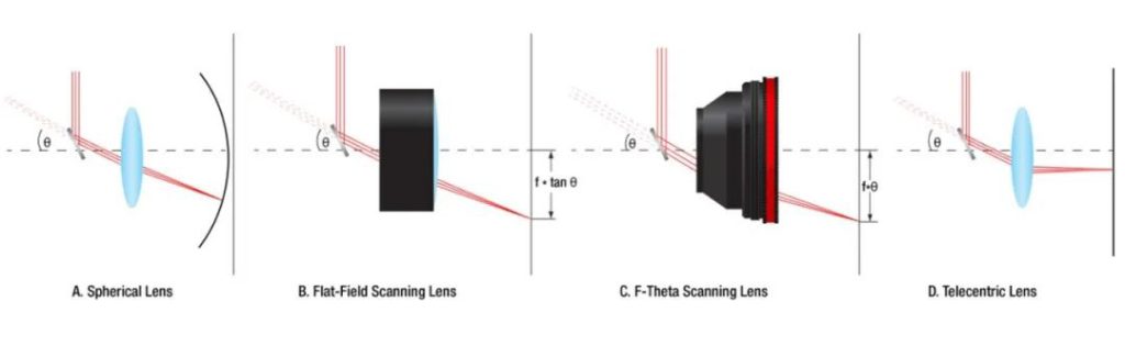
Most scanning lenses are of the fθ correction type. This is because the focal plane of a simple spherical lens is a curved surface. Although a flat field lens can correct field curvature, the distance between its focal point and the scanning angle are not linearly related and are not an ideal choice. Additionally, some scan engines use telecentric lenses to focus the light perpendicular to the image plane. This allows the beam to pass efficiently through the optics without escaping outside the system periphery. Important specifications for a scanning lens are focal length, entrance pupil diameter, field number, and design wavelength range.
Tube lenses also have focal length to focus on first, as it affects the magnification of the scan engine. The second is the field of view of the intermediate image plane between the scanning lens and the tube lens. The fields of view of these two lenses must match to achieve high-efficiency scanning. The third is the entrance pupil diameter, which actually refers to the pupil on this side of the objective lens. It must be as large as the rear aperture of the objective lens. The fourth is the design wavelength range.
There are two types of scanning mirrors: Resonance Scanning Mirror (Resonance Mirror) and Galvo Mirror (Galvo Mirror). The former is used for rapid scanning parallel to the x-axis, and the latter is used to advance line by line and provide return travel.
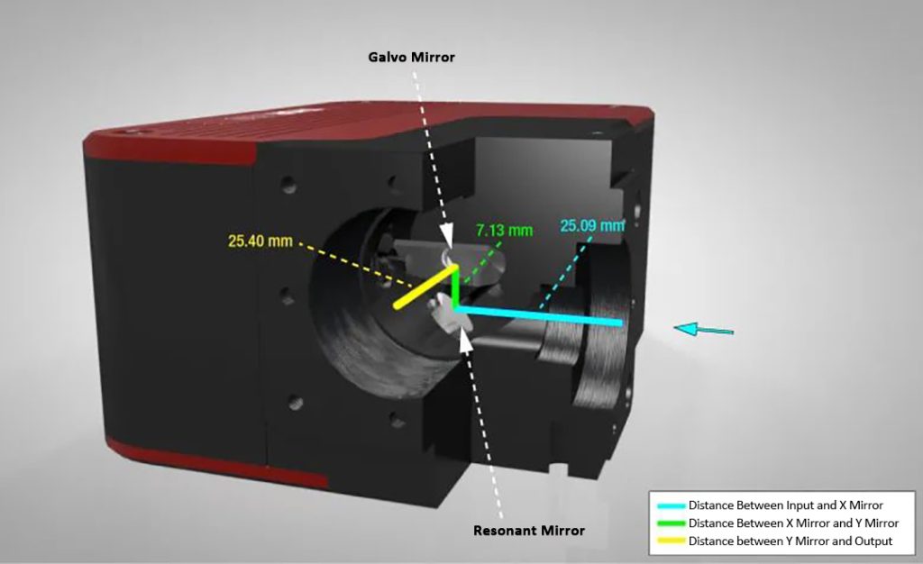
Galvo mirrors can accurately control the scanning position, but their speed and acceleration are relatively slow, and their size and speed are mutually restrictive. The size of the beam transmitted by the scan engine is limited by the size of the scanning mirror, but using large mirrors will reduce speed. Resonance mirrors are fast and have a sinusoidal relationship between angle and time. Resonance sweeps can only control amplitude, and higher frequencies will slightly reduce the amplitude.
Scanning mirrors are usually integrated in two axes into a scan head. Galvo-Galvo scanner and Galvo-Resonance scanner are two common configurations. The galvanometer scanner can scan any point in the field of view and stay for any time, and can also scan any shape, but it is slow. Resonance scanners are fast, but they can only scan squares, rectangles or straight lines, and they must scan along the axis.

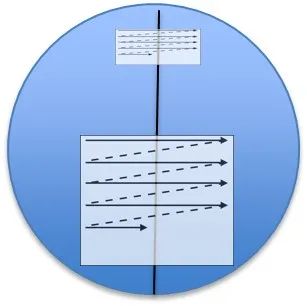
The galvanometer scanner has limited acceleration and needs time to decelerate, so it will exceed the field of view by a large amount. The lower left image shows an image intentionally bleached using a galvanometer scanner. The yellow box represents the imaging area, but it is obvious that the actual scan extends from both sides.
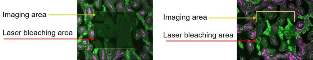
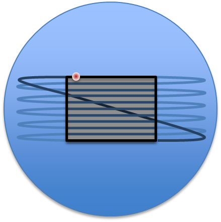
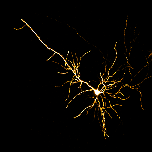
The residence time of the resonance scanner at different positions varies greatly. The upper right picture is an image collected by an 8kHz resonance scanner. The dwell time in the middle of the field of view is about 0.1 μs, and the dwell time at the edge exceeds 2 μs. Because the scanning dwell time is very short, the sample is not easily bleached. Look carefully at the two dark lines in the picture. Using a high-speed power modulation device can turn off the laser at the edge of the field of view and reduce sample damage.
Laser scanning detectors need to be fast, typically with a dwell time of less than 0.1 μs at each pixel, and require a large sensor area to capture as many photons as possible. Photomultiplier tubes are the traditional choice for laser scanning microscopy. They offer nanosecond rise and fall times as well as high dynamic range and low readout noise, but the disadvantage is that the maximum quantum efficiency is only about 40%.
Alternatives to photomultiplier tubes include avalanche photodiodes. Although this kind of detector has higher quantum efficiency and is very fast, it has a low dynamic range and may be damaged beyond very low light intensity ranges. In recent years, silicon photomultiplier tubes have made great progress.
Confocal scan engine
The purpose of confocal is to suppress light outside the focus, resulting in a clearer image. This is because if the sample is thick, out-of-focus light hitting the detector will blur the image. The implementation method of confocal is to add a pinhole to the image plane, so that only the sample light from the focal plane can be focused on the pinhole through the scan engine and enter the detector. Light outside the focal point is mostly blocked by the outside of the pinhole.
Below is a dynamic image of confocal scanning and detection. The entire system is suitable for both the center point of the field of view and other points in the focal plane. When the scanning mirror is deflected and the laser excites the sample off-axis through the scan engine, the emitted light remains accurately focused on the pinhole along the exact same path through the dichroic mirror.

Confocal reconstructs 3D images via Z-stack
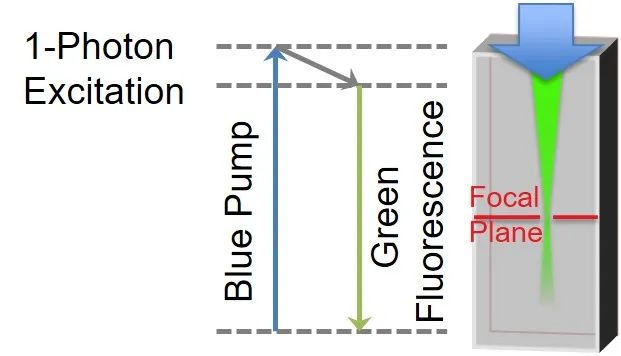
Below the multiphoton scanning engine are electron energy level diagrams for single-photon and two-photon imaging. For single-photon imaging, a high-energy blue photon jumps a ground-state electron to an excited state, then relaxes to a slightly lower energy level during the fluorescence lifetime, and finally returns to the ground state from there and emits a slightly lower-energy green photon.
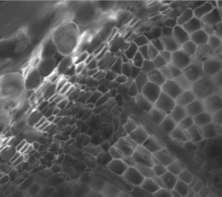
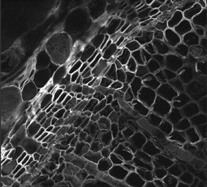
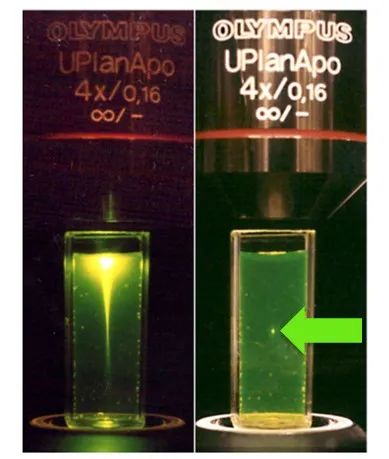
Comparison of single-photon and two-photon imaging of actual samples
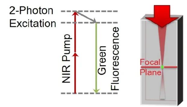
For two-photon imaging, two low-energy near-infrared photons can achieve the same transition process as the above-mentioned blue light, but the energy of the emitted photon is higher than that of the near-infrared photon. Two-photon excitation requires a pulsed laser with high peak power to achieve.
Multiphoton imaging can image deeper into tissue because it uses long wavelengths, and provides natural optical sectioning capabilities. In the comparison image below, the excitation area for single-photon imaging is hourglass-shaped, while only the bright light at the focus is visible for two-photon imaging. This is because two-photon excitation can only be achieved if the photon density at the focus is high, so this is an inherent optical section that does not produce fluorescence outside the focus and does not require the addition of pinholes.
Although ideally, the detector would surround the sample with a spherical surface to collect all the light, most multiphoton microscopes collect only through the objective lens. Different from the confocal detection method (De-scanned), the multi-photon microscope uses a dichroic mirror directly after the objective lens to allow the fluorescence to enter the detector through the collection lens.